How to easily perform the Haigis triple optimization

The Haigis Formula

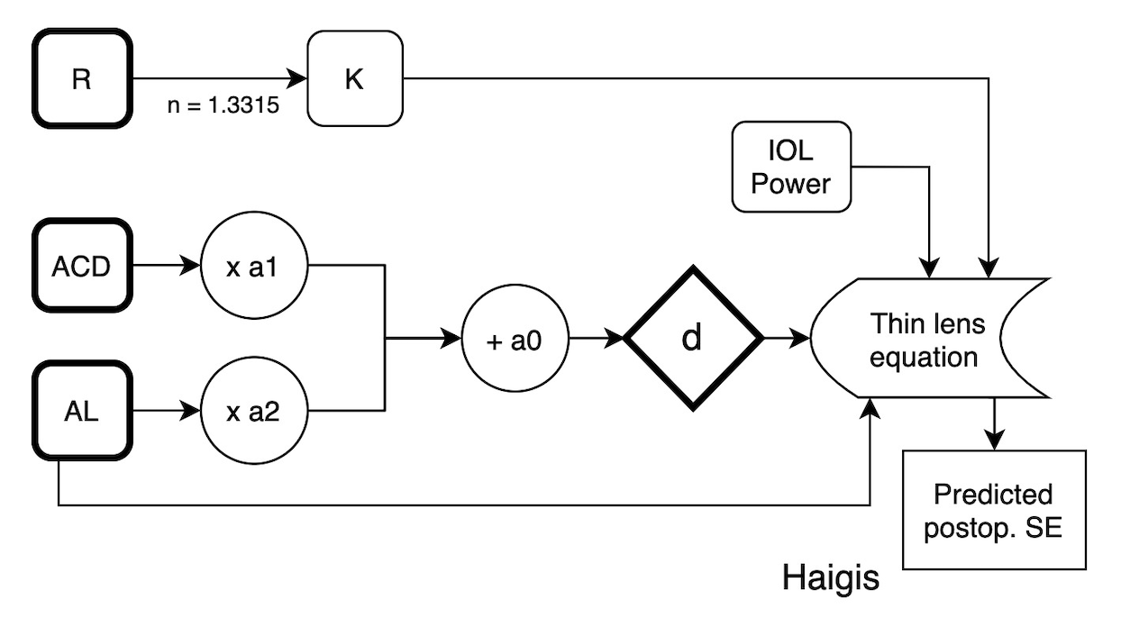
The Haigis formula is the simplest thin lens formula possible. The ELP (= d value) is predicted using a multiple regression taking ACD and AL as inputs.

def Haigis(AL, R, ACD,a0,a1,a2,power): 
    n = 1.336 
    nc = 1.3315 
    dx = 0.012 
    d = a0 + a1*ACD + a2*AL 
    R = R/1000 
    AL = AL/1000 
    d = d/1000 
    Dc = (nc - 1)/(R) 
    qnum = n * (n - power * (AL - d)) 
    qdenum = n * (AL - d) + d * (n - power *(AL-d)) 
    q = qnum / qdenum 
    SEpred = round((q - Dc) / (1 + dx*(q - Dc)),3) 
    return SEpred

Optimizing the Haigis Formula

The Haigis formula can be single-optimized (A0 acts like a "potentiometer" or variable resistor, like the A constant in SRK/T, until a mean prediction error equal to zero is reached) or triple-optimized.

The Haigis triple-optimization is in fact a complete retraining of the formula. The perfect d value is back-calculated for each eye of the dataset. This is the d value giving the real postoperative spherical equivalent when using the biometric values and the implanted IOL power in thin lens equations.

A multiple regression takes ACD and AL as inputs, then allows fitting to predict this "perfect" d value. Et voilà : the intercept is a0, the ACD coefficient is a1, and the AL coefficient is a2.

Back-calculation of the d value

You can back-calculate the d value for a given eye with the following function (As expected you'll need the postoperative SE, ARC, AL and the implanted IOL power).

# AL, R in meters 
def solve_d_Haigis(AL, R, power, Rx): 
    n = 1.336 
    nc = 1.3315 
    dx = 0.012 
    Dc = (nc - 1) / R 
    z = Dc + Rx/(1-Rx*dx) 
    b = -power * (AL + n/z) 
    c = (n * (AL - n/z) + power * AL * n/z) 
    d = (1 / (2*power)) * (-b - np.sqrt(b**2 - 4 * power * c) ) 
    return d

From :  W.Haigis. "The Haigis formula", in Intraocular Lens Power Calculation, H. John Shammas, Chapter 5, edited by  Slack Incorporated, 2004.

# Example : 

val = solve_d_Haigis(0.024, 0.0075, 21, -2) 
print(val) 

#output : 0.005461457048808832

The output of this function is in meters : multiply by 1000 before fitting your regression.

Like this :

from sklearn.linear_model import LinearRegression
df['d_Haigis'] = df['d_Haigis'] * 1000
lin = LinearRegression()
lin.fit(df[['ACD','AL']], df['d_Haigis'])
lin.intercept_

# output : 
# -0.07756916259537494

This is your a0 value !

lin.coef_

# output : 
# array([0.39819972, 0.16012471])

And the coefficients are a1 and a2, respectively. What a beautifully simple formula! Genius.